Earth Science · ESS-001
Earthquake Epicenter
Seismometers find where a quake started — and what lies deep inside Earth.
- NGSS HS-ESS2-3
- NGSS HS-PS4-1
- AP Environmental Science Unit 4
Included with a subscription. Create a free account to get started.

About this lab
Pick seismic wave arrivals from station records and locate the earthquake represented by them. In this interactive 3D investigation for high school students, inspect local or global records, place arrival markers, and use the travel-time information to construct distance circles around the observing stations. The map comparison combines the circles with an origin-time calculation and uncertainties in the picked arrivals. Earth's cutaway view displays ray paths, changes across internal boundaries, and missing-wave regions. These observations connect the station measurements with evidence about the planet's layered interior. These activities are aligned with NGSS HS-ESS2-3, NGSS HS-PS4-1, and AP Environmental Science Unit 4.
The question behind the experiment
A seismogram records when different seismic waves reach a station, not a direct map of where an earthquake began. This course turns arrival-time evidence into a location estimate. Identify the first P-wave and S-wave arrivals before drawing distance circles. Their time separation carries information about the path traveled. A larger signal is not automatically evidence of a more distant earthquake, so keep arrival timing distinct from amplitude when explaining how the investigation works.
Plan a useful comparison
Pick the two arrivals on the same station record and retain their times with the instrument's resolution. Convert the S–P interval using the travel-time relationship appropriate to the selected scale. The course distinguishes a local constant-speed calculation from a global travel-time curve. A global curve can be curved because Earth's interior is layered and the rays follow different paths. Applying a single local speed to every distance would hide the assumptions in your estimate.
Connect the observation to the model
Draw a circle centered on each station with the estimated epicentral distance as its radius. A station constrains the epicenter to a ring rather than identifying a unique location. Additional stations narrow the candidates. Compare your placed estimate with the circle intersections and the fit supplied after the investigation's prediction steps. If the circles do not meet perfectly, describe the mismatch rather than forcing an exact crossing. Both arrival picking and the assumed velocity structure can contribute.
Interpret the result carefully
The origin time is another inference, separate from the arrival time shown at a station. Subtract the estimated P-wave travel time from the observed P arrival to infer when the earthquake started. Keep clock times and elapsed travel times in separate columns. A plausible location can still accompany an incorrect origin-time calculation if those quantities are mixed. Use the same travel-time model for the distance and time inference so the two results refer to compatible assumptions.
Build an explanation from your evidence
The interior view connects the location exercise to a layered Earth model. Compare which waves travel through each region and where shadow zones occur. The absence of ordinary S-wave transmission through a liquid outer core is evidence about material properties, not proof that seismic energy simply disappears. Use the model to relate the travel paths to station observations. This course explores seismic evidence and uncertainty; its teaching scenarios are not a live earthquake warning or hazard forecast.
A reference case from this course
At an epicentral distance of 5000 km, the specified travel-time reference gives P arrival after 496.7 s and S arrival after 896.9 s, an S–P interval of 400.2 s. These elapsed times belong to the course velocity model. They illustrate the conversion chain and do not describe every earthquake at that distance.
Keep the investigation reproducible
Before changing the setup, write a prediction that names the measured quantity and the expected direction of change. Retain the original trial as a reference. Record the apparatus conditions, units, and whether you used Ideal or Real lab mode. If the selected activity includes seeded variation, keep the seed and run identity with the result so another comparison does not silently mix different conditions.
Separate the observation from its explanation. A reading or a counted object belongs in the evidence; the relationship you use to interpret it belongs in the reasoning. When a result differs from the reference case, check the settings and measurement procedure before deciding that the model relationship has failed. Describe a specific source of uncertainty and where it enters your calculation. Finish with a claim supported by the recorded comparison, and identify an additional trial that could distinguish your explanation from an alternative.
Continue the comparison
Follow the geographic context in Plate Tectonics & Seafloor Spreading, or revisit wave timing in Ripple Tank Waves. Compare the evidence each model uses before transferring an explanation from one scale to the other.
Common questions
Standards alignment
- NGSS HS-ESS2-3
- NGSS HS-PS4-1
- AP Environmental Science Unit 4
More Earth Science labs
- Members
Earth Science
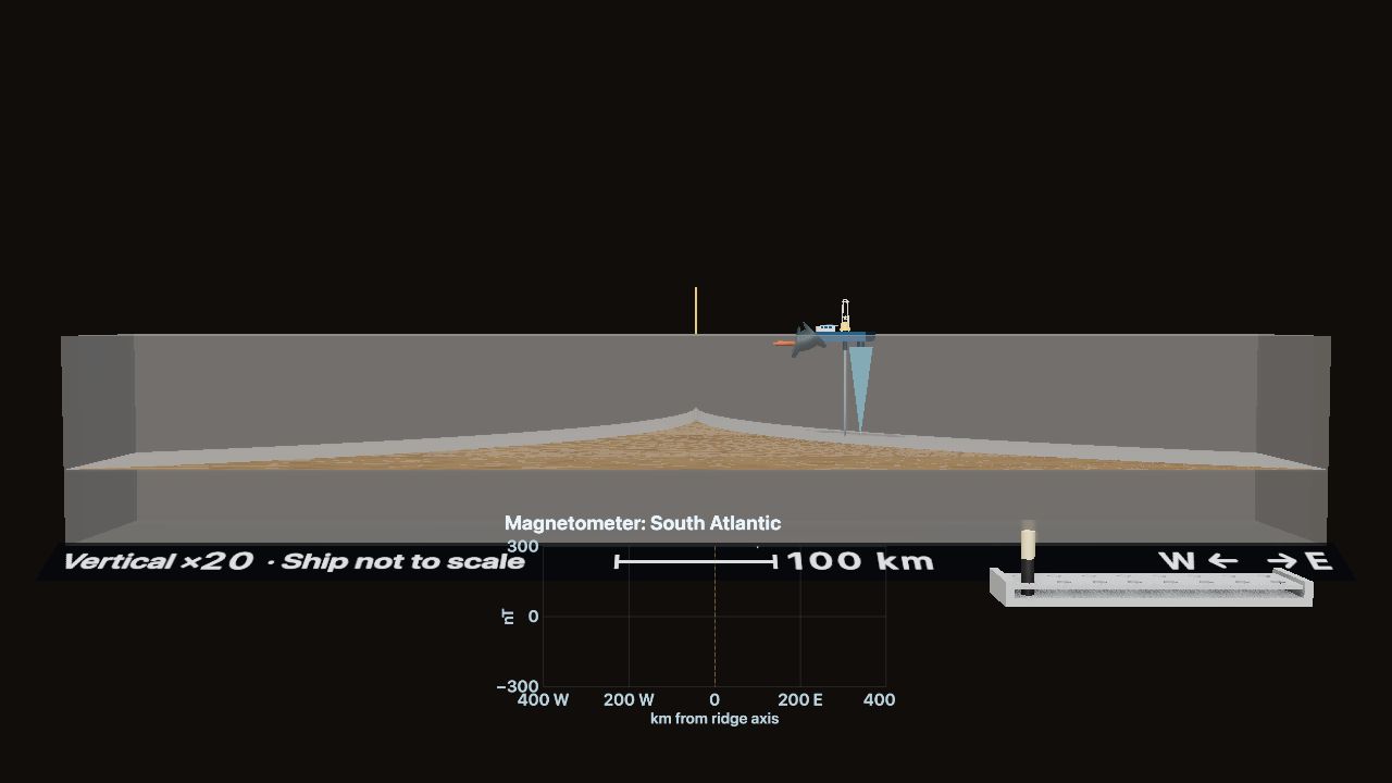
Seafloor Spreading & Plate Boundaries
Tow a magnetometer and drill cores across a mid-ocean ridge. What record do the seafloor rocks keep?
- Members
Earth Science
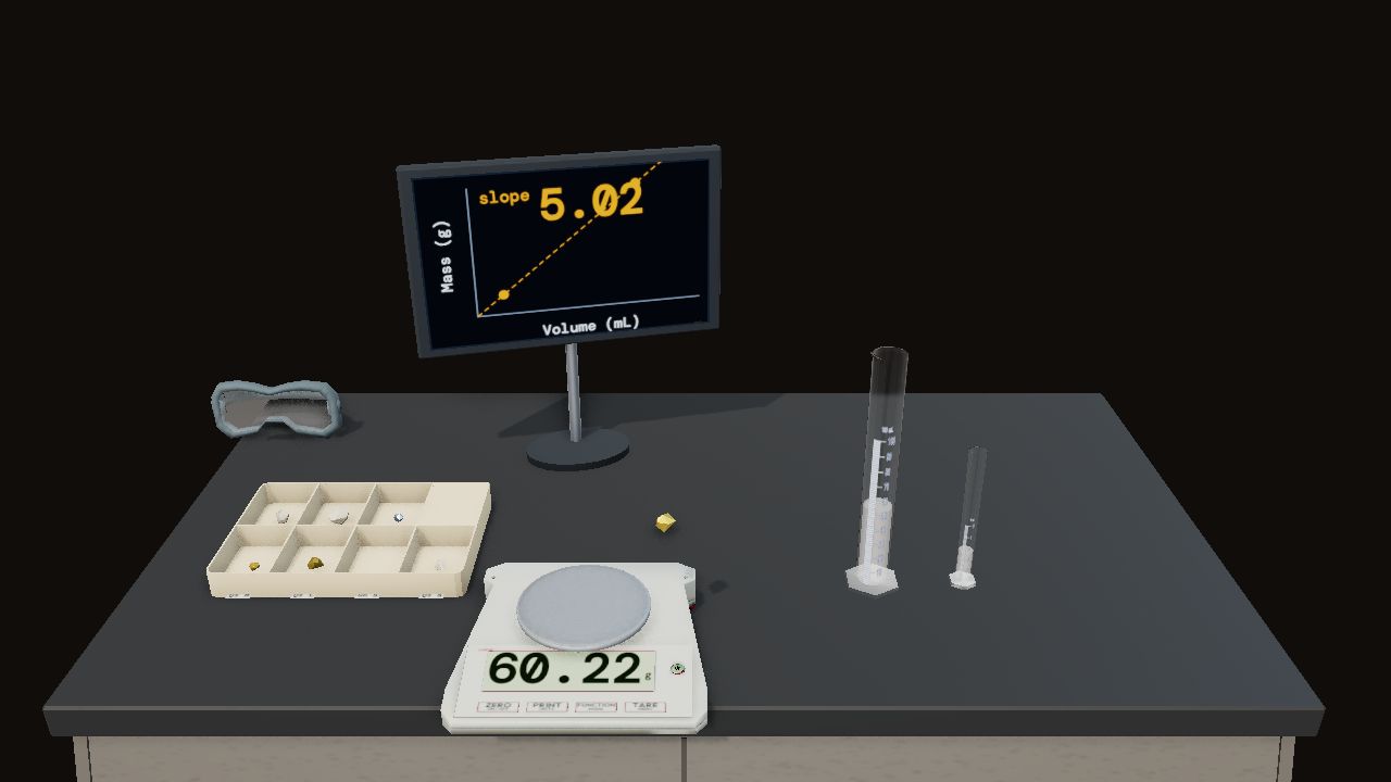
Mineral & Rock Identification
Scratch, streak, and split unknown specimens. Name the mineral, then the rock.
- Members
Earth Science
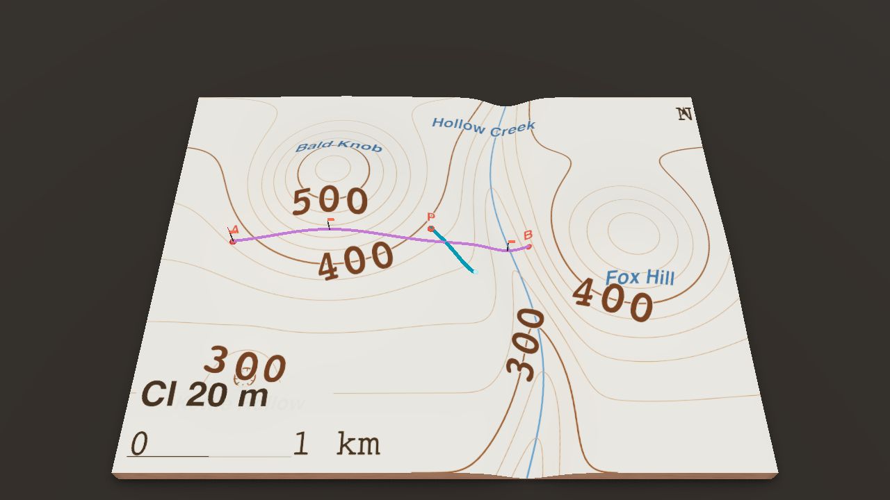
Topographic Maps & Landforms
Match contour lines to hills and valleys, then draw a profile.


